Mean time between failures
Mean time between failures (MTBF) is the predicted elapsed time between inherent failures of a system during operation.[1] MTBF can be calculated as the arithmetic mean (average) time between failures of a system. The MTBF is typically part of a model that assumes the failed system is immediately repaired (MTTR), as a part of a renewal process. This is in contrast to the mean time to failure (MTTF), which measures average time to failures with the modeling assumption that the failed system is not repaired (infinite repair rate).
The definition of MTBF depends on the definition of what is considered a system failure. For complex, repairable systems, failures are considered to be those out of design conditions which place the system out of service and into a state for repair. Failures which occur that can be left or maintained in an unrepaired condition, and do not place the system out of service, are not considered failures under this definition.[2] In addition, units that are taken down for routine scheduled maintenance or inventory control, are not considered within the definition of failure.
Contents |
Overview
For each observation, downtime is the instantaneous time it went down, which is after (i.e. greater than) the moment it went up, uptime. The difference (downtime minus uptime) is the amount of time it was operating between these two events.
MTBF value prediction is an important element in the development of products. Reliability engineers / design engineers, often utilize Reliability Software to calculate products' MTBF according to various methods/standards (MIL-HDBK-217F, Telcordia SR332, Siemens Norm, FIDES,UTE 80-810 (RDF2000), etc.). However, these "prediction" methods are not intended to reflect fielded MTBF as is commonly believed. The intent of these tools is to focus design efforts on the weak links in the design.
Formal definition of MTBF
By referring to the figure above, the MTBF is the sum of the operational periods divided by the number of observed failures. If the "Down time" (with space) refers to the start of "downtime" (without space) and "up time" (with space) refers to the start of "uptime" (without space), the formula will be:

The MTBF is often denoted by the Greek letter θ, or
The MTBF can be defined in terms of the expected value of the density function ƒ(t)
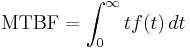
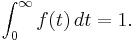
where ƒ is the density function of time until failure – satisfying the standard requirement of density functions –
Common MTBF misconceptions
MTBF is commonly confused with a component's useful life, even though the two concepts are not directly related. For example a battery may have a useful life of four hours, and an MTBF of 100,000 hours. These figures indicate that in a population of 1,000,000 batteries, there will be approximately ten battery failures every hour during a single battery's four-hour life span.[3]
Another common misconception about the MTBF is that it specifies the time (on average) when the probability of failure equals the probability of not having a failure (i.e. an availability of 50%). This is only true for certain symmetric distributions. In many cases, such as the (non-symmetric) exponential distribution, this is not the case. In particular, for an exponential failure distribution, the probability that an item will fail at or before the MTBF is approximately 0.63 (i.e. the availability at the MTBF is 37%). For typical distributions with some variance, MTBF only represents a top-level aggregate statistic, and thus is not suitable for predicting specific time to failure, the uncertainty arising from the variability in the time-to-failure distribution.
Another misconception is to assume that the MTBF value is higher in a system that implements component redundancy. Component redundancy can increase the system MTBF, however it will decrease the hardware MTBF, since, generally the greater number of components in a system, the more frequent a hardware component will experience failure, leading to a reduction in the system's hardware MTBF.[4]
Variations of MTBF
There are many variations of MTBF, such as mean time between system aborts (MTBSA) or mean time between critical failures (MTBCF) or mean time between unit replacement (MTBUR). Such nomenclature is used when it is desirable to differentiate among types of failures, such as critical and non-critical failures. For example, in an automobile, the failure of the FM radio does not prevent the primary operation of the vehicle. Mean time to failure (MTTF) is sometimes used instead of MTBF in cases where a system is replaced after a failure, since MTBF denotes time between failures in a system which is repaired.
Notes
- ^ Jones, James V., Integrated Logistics Support Handbook, page 4.2
- ^ Colombo, A.G., and Sáiz de Bustamante, Amalio: Systems reliability assessment – Proceedings of the Ispra Course held at the Escuela Tecnica Superior de Ingenieros Navales, Madrid, Spain, September 19–23, 1988 in collaboration with Universidad Politecnica de Madrid, 1988
- ^ Vargas, E., Bianco, J.,Deeths D., Sun Cluster Environment Sun Cluster 2.2, Prentice Hall PTR; 1st edition (April 4, 2001), ISBN 0130418706
- ^ Vargas, E., Bianco, J.,Deeths D., Sun Cluster Environment Sun Cluster 2.2, Prentice Hall PTR; 1st edition (April 4, 2001), ISBN 0130418706
See also
References
- Jones, James V., Integrated Logistics Support Handbook, McGraw–Hill Professional, 3rd edition (June 8, 2006), ISBN 0071471685